Review of Professional Management

 Search

Rakesh Shahani1 and Kartikay Ahluwalia1
1Department of Business Economics, Dr. Bhim Rao Ambedkar College, University of Delhi, India

Creative Commons Non Commercial CC BY-NC: This article is distributed under the terms of the Creative Commons Attribution-NonCommercial 4.0 License (http://www.creativecommons.org/licenses/by-nc/4.0/) which permits non-Commercial use, reproduction and distribution of the work without further permission provided the original work is attributed.
Purpose: The study makes an attempt to investigate the long-term dynamic relation between CO2 emissions from liquid fuel consumption by the transport sector (TR) and the ecological footprint (EFP) of two Asian emerging giants, namely, China and India. Four other variables, ‘Urbanisation’, ‘Trade Openness’, ‘ICT’ and ‘GDP’ have also been included under the study as control variables. The period of study is 30 years (1987–2016), and the data have been sourced from World Development Indicators and Global Footprints Network.
Methodology: The methodology includes testing for co-integration amongst variables by applying the ARDL co-integration model (with a single breakpoint) and its non-linear counterpart, NARDL. The error correction, testing for asymmetric impact and long-run elasticity are other aspects considered under the study.
Findings: Co-integration was established at 1% level for both countries, both under the ARDL and NARDL models. The long-run impact of TR on EFP was positive for both countries, with elasticity between TR and EFP being highly inelastic for India and somewhat elastic for China. The asymmetric impact of TR on EFP was not seen in either of the two countries in the long run. The long-run adjustment process through the ECM(–1) term was found to be stable, but the speed of adjustment was moderate @7% p.a. for China and slow @0.3% p.a. for India. All three model diagnostics were found to be highly satisfactory.
Study Implications: Adjustment speed at 7% p.a. for China and 0.3% p.a. indicates that for India, the long-run relation between TR and EFP would only be reached after a few years, which gives sufficient time for the policy makers to act towards deciding on the roadmap to sustainable development. Then, for India, the elasticity between TR and EFP was inelastic in the long run; this was fairly elastic for China, which implied that China was strategically better placed and well prepared for the transformation to renewable energy to run the TR, while India may have to continue with the traditional fuels for some more time.
ARDL, asymmetry, co-integration, ecological footprint, NARDL
Introduction
Fossil fuels, central to manufacturing, are a major driver of economic growth in both resource-rich and resource-scarce economies. Transport, which serves as a catalyst in economic growth, has experienced significant expansion over recent decades, making this sector a leader in energy consumption, accounting for about 25% of global GHG emissions in 2021 (UN Fact Sheet, 2021). This surge, fuelled by globalisation, urbanisation, and trade, has intensified fossil fuel use and environmental degradation. With only 3.7% of its energy from renewables and 96.3% from fossil fuels, immediate regulatory actions and investment in sustainable infrastructure are highly critical, and hence the sector requires the highest priority (IRENA, 2021).
Global efforts to cut fossil fuel use in transport have shown promise but remain concentrated in developed nations. For example, a US study (1977–2007) by Brown-Steiner et al. (2016) found black carbon emissions from diesel trucks and trains dropped despite rising freight volumes, thanks to policies like transport clustering and regulatory enforcement. Nonetheless, such progress is limited in developing countries.
Despite evident environmental harm, many nations hesitate to act due to the substantial investment required for cleaner fuels and economic significance of the transport sector (TR) in enhancing productivity, employment, property values and other benefits (Pradhan et al., 2024). Scholars suggest non-conflicting policies, which demand understanding the interplay among growth, energy, and CO2 emissions.
Beyond GHGs, transport also causes noise pollution and waste generation. According to OECD (2021), transport’s energy share is highest in the US (37.5%), UK (33%), and Switzerland (31%), compared to 15% in India and China, which actually contradicts developed economies taking proactive measures to combat transport emissions. Within transport, road transport accounts for about 75% of CO2 emissions, the rest being shared by air and rail (Saboori et al., 2014). In emerging economies, industrial energy use remains high—China (49%), Indonesia (37%), India (38%), while in developed nations it has fallen significantly—US (17%), UK (18%) (IRENA, 2021). This points to a relocation of energy-intensive industries from developed to developing countries.
Shifting the focus to the present study, leaving aside overall emissions, research reveals that sector-specific energy consumption remains largely unexplored. Although for emissions, most studies have considered CO2 or SO2 emissions as their proxy for environmental degradation, the sector-wise breakup of these emissions has been largely ignored, which becomes one of the motivations of the present study.
The study investigates the long-run relationship between transport emissions and environmental degradation in two emerging Asian economies, China and India, the criterion for sample choice being their rapid economic growth amongst developing nations. The study employs ecological footprint (EFP) and liquid fuel consumption by transport as main proxies besides four control variables: Urbanisation, trade openness, ICT, and GDP. Including control variables prevents omission bias and aligns the study with previous studies (Frey et al., 2006; Hassan et al., 2019). A 30-year dataset, log-transformed, is used for analysis. EFP data from the Global Footprint Network (2023) covers six land categories and reflects the environmental cost of production and waste, adjusted for Earth’s regenerative capacity (Nathaniel & Khan, 2020; Rashid et al., 2018).
Strand et al. (2021) report that rising global EFP is driven by poor natural resource management and weak environmental regulation. Innovation in technology is cited as a key solution to reversing ecological degradation. Santos (2017) links regulatory failure to the absence of a global enforcement body.
Before discussing methodology, the study reviews relevant literature, categorised into two groups: Studies analysing transport emissions and studies examining related control variables. The impact of some of the control variables on the environment has been found to be country-specific, for example, most studies find that urbanisation’s environmental effects are country-specific—harmful in China and Qatar (Charfeddine, 2017; Sheng & Guo, 2016), but beneficial in the UAE and MENA countries (Charfeddine & Ben Khediri, 2016; Charfeddine & Mrabet, 2017). On the other hand, ICT, often measured by mobile usage or subscriptions, is generally linked to lower environmental degradation. For instance, Salahuddin et al. (2016) found mobile use was negatively related to CO2 in OECD countries, while Asongu et al. (2017) found similar results in Sub-Saharan Africa. Hussain et al. (2023) showed that ICT combined with urbanisation and electricity use reduced EFP. Contrastingly, in Iran, ICT increased industrial CO2 emissions (Shabani & Shahnazi, 2019). Then, the existence of an asymmetric impact of ICT on emissions was reported in a study on Tunisia (Amri et al., 2019).
Studies focusing on the main variable, transport emissions, include Brown-Steiner et al. (2016), who showed reduced emissions through policy and enforcement. Others, including Ayadi and Hammami (2015) and Sasana and Aminata (2019), stress that without strong regulation, environmental damage is unavoidable. Abbes and Bulteau (2018) found that transport accounted for 92% of Tunisia’s GHG emissions.
Transport energy consumption was found to be closely linked to CO2 emissions in many studies. A study by Nasreen et al. (2020) found bidirectional relationships between CO2 and transport energy in 18 countries. Saboori et al. (2014) showed long-run, positive links among CO2, economic growth, and road sector energy use across OECD countries. The study showed that impulses of road sector energy consumption towards CO2 emissions lasted longer than impulses towards economic growth, implying long-run policies could be framed for shifting to renewable fuels and could benefit in mitigating GHG emissions.
With respect to the relation between transport and EFP, there have been only a handful of studies, like Hussain et al. (2023), which showed that a reduction in EFP was possible by increasing expenditure on transport infrastructure and through sustained economic growth. Then, Satrovic et al. (2024) concluded that transport energy and natural resource depletion were responsible for the rise in EFP, while technological innovation was seen as reducing the same.
Then, apart from emissions, another TR variant becoming popular amongst researchers is transport infrastructure and the same was considered in studies including Churchill et al. (2021), Pradhan et al. (2024), Acheampong et al. (2022), amongst others. The variable transport infrastructure with both positive and negative multiplier effects, positive in terms of saving travel time and costs, increasing employment (Pradhan et al., 2024), while negative being the use of environment-unfriendly products; cement, concrete and heavy-duty equipment by infrastructure projects themselves. Churchill et al. (2021) found that a 1% rise in transport infrastructure was associated with a 0.4% rise in CO2 emissions.
Research Gap
The literature review revealed limited studies examining the role of control variables while modelling the transport-environment relation, particularly in emerging markets. This study fills the gap by including such control variables to bring out the deterministic role played by each and every control factor towards the environment, even though the study objective was to establish the relation between transport emissions and EFP. Furthermore, the review apprised us that the research area, transport emissions and EFP linkages was highly under-researched as the study could figure out only a few studies alongside developed economies. The study, which includes India and China, two developing economies, would try to compare the outcome of the current research with the outcome in developed economies.
A unique feature of this study was its dual modelling approach using both quasi-linear ARDL (with structural break) and non-linear NARDL models. This methodology choice stems from the BDS test results, which indicated non-linear behaviour in EFP. While ARDL models (Pesaran et al., 2001) would handle mixed-order integration, assuming linearity by incorporating structural breaks, NARDL tends to focus on nonlinearities (Shin et al., 2014), allowing better modelling of complex dynamics. To the best of our knowledge, no study has applied both ARDL variants to explore this relationship.
The rest of the article is structured as follows: The second section presents descriptive statistics, the third section explains the methodology employed, the fourth section provides empirical results, and finally, the fifth section presents a conclusion, study limitations and policy implications, followed by references in the sixth section.
Summary Information and Descriptive Statistics of the Variables
Table 1 summarises the six variables along with their units of measurement and data sources, and is shown under three columns, sources of data being the World Bank (2023) and Global Footprints Network (2023). Table 2 compares descriptive statistics of these variables for India and China over the 30-year period (1987–2016). China’s average EFP was four times India’s, with CO2 emissions from transport in China being about 2.2 times higher. For the four control variables, China also consistently reported higher averages.
Table 1. Summary Information About the Variables Included in the Study.
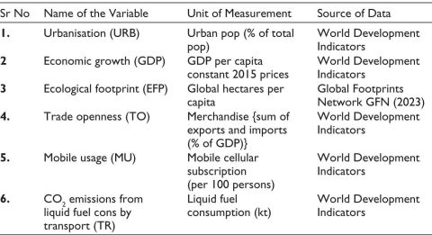
Table 2. Statistical Description of Variables for the Period 1987–2016.
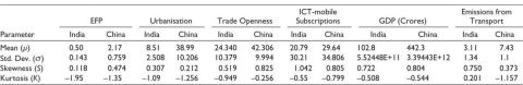
Standard deviation, which indicates variability, was higher for China for five out of six variables. India showed more variability only in TR emissions, suggesting inconsistent trends compared to China’s more stable emission control. Skewness results showed a strong positive skew for China’s EFP, implying more years with values above the average. India’s EFP also had a positive skew, but less pronounced, suggesting a more balanced distribution. India’s TR skewness was much higher than China’s, indicating frequent years of emissions above the average. Kurtosis values were negative for most variables, indicating flatter, more normal-like distributions, suggesting no large distribution asymmetries for either country.
In summary, Table 2 gives preliminary insight into the trends of two emerging economies. For India, TR emissions seem to be a major driver of EFP changes, while in China, other sectors such as industry and power may be more responsible. This aligns with findings by Shang et al. (2024), who observed that China’s emissions reduction came from a gradual switch to low-carbon fuels, thereby taking the burden off the TR.
Methodology
The methodology revolves around two co-integration variants: ARDL with a single structural break and NARDL, choice being based upon results obtained under the BDS test statistics. Hence, before any discussion on the two variants, the study explores the methodology employed for the BDS test statistics.
BDS Test
BDS test statistic (Brock et al., 1987) determines whether data is independently and identically distributed (I.I.D), and the study has applied BDS on raw data with ‘m’ embedded dimension with histories being rolled over in the following manner:

Null Hypothesis
H0: I.I.D. time series data.
HA: Time series data is not I.I.D.; hence, non-linear
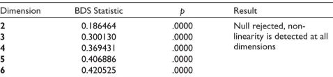
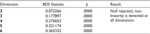
Based upon the BDS results obtained (shown under Table 3), we decided to develop two models: ARDL with a single structural break and NARDL. Further, with non-linearity being proved, the study introduced a Dummy variable for the dependent variable in the ARDL model, thus making this model a quasi-linear model.
Table 3. BDS Results for Our Variable EFP (China).
Model Representation (ARDL with Single Structural Break)
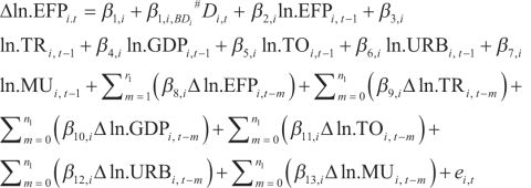
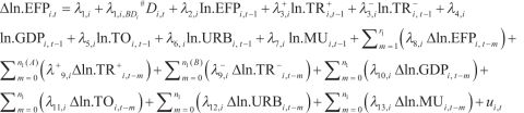
The section discusses the ARDL co-integration Model with a single structural break for the variable EFP; model representation for the same is given as Equation 1.
 (1)
(1)
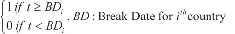
For Equation 1, Δln.EFPi,t is the logarithmic change in EFP, model dependent variable, with ‘t’ being the time period and ‘i’ representing two countries; i = 1, 2, 1 (India) or 2 (China). Equation 1 has ‘.png) 1’as intercept while ‘1, t#’ slope coefficient of Intercept Dummy (D1) reflecting structural break of dependent variable, EFP. As stated above, the inclusion of a structural break is based upon the BDS test results and applies Perron’s Innovative Outlier Method (Perron, 1994), following asymptotic one-sided ‘p’ values. Dummy Variable (Di,t) takes the value as:
1’as intercept while ‘1, t#’ slope coefficient of Intercept Dummy (D1) reflecting structural break of dependent variable, EFP. As stated above, the inclusion of a structural break is based upon the BDS test results and applies Perron’s Innovative Outlier Method (Perron, 1994), following asymptotic one-sided ‘p’ values. Dummy Variable (Di,t) takes the value as:
‘2’ is the slope coefficient of the first lag of dependent variable EFP, while next five terms, ‘3’ to ‘7’ are slope coefficients of first lag of five independent variables, namely, TR, GDP, URB, TO and MU, respectively. Five further independent variables at their first lags together with the dependent variable EFP make up the long-term relation under ARDL.
The term .png) depicts log change in dependent variable EFP and has been included as a regressor, with ‘r1’ being AIC determined lags. Similarly, the term for transport is
depicts log change in dependent variable EFP and has been included as a regressor, with ‘r1’ being AIC determined lags. Similarly, the term for transport is .png) , ‘n1’ being the lags (AIC), and the same goes for other independent variables. Further, with a limited number of observations under study, a restriction of Max ‘2’ lags for both dependent and independent variables was considered, that is, m = Max of Lags (0,1,2) for independent and m = Max of Lags (1,2) for dependent variable. These terms are then summed up and collectively make up the short-run relation. Finally, ei,t is the stochastic error term of Equation 1.
, ‘n1’ being the lags (AIC), and the same goes for other independent variables. Further, with a limited number of observations under study, a restriction of Max ‘2’ lags for both dependent and independent variables was considered, that is, m = Max of Lags (0,1,2) for independent and m = Max of Lags (1,2) for dependent variable. These terms are then summed up and collectively make up the short-run relation. Finally, ei,t is the stochastic error term of Equation 1.
Model Representation (NARDL)
NARDL model (Shin et al., 2014) is an asymmetric expansion of ARDL and decomposes our independent variable, TR, into positive and negative values, keeping rest of the variables unchanged as given under Equation 1. NARDL model for dependent variable EFP is given as Equation 2 below:
 (2)
(2)
where
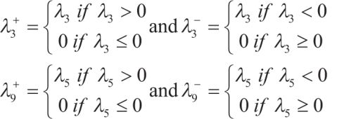
As already stated, the variable TR in Equation 2 is decomposed as TR+ and TR–, TR+ takes a positive value when variable TR is positive, while for all zero and negative values of variable TR, TR+ takes a value as ‘0’. Again, variable TR– takes a negative value if TR is negative, while for all other values of TR, TR– takes a value as ‘0’.
Test for Long-term Co-integration: Partial ‘F’ Bounds Test
The existence of co-integration under both models is tested by applying partial ‘F’ bounds test (Pesaran et al., 2001). We set up two null hypotheses, one for ARDL and the second for NARDL, under ‘F’ bounds test
HO1: 2 = 3= 4 = 5 = 6 = 7 = 0 (for ARDL Equation 1)
HO2: .png) 2 = 3= 4 = 5 = 6 = 7 = 0 (for NARDL Equation 2)
2 = 3= 4 = 5 = 6 = 7 = 0 (for NARDL Equation 2)
Null gets rejected if ‘F’ computed > Upper Bound critical (Table 5)
Long-term Relation: Elasticity and Asymmetry
The section discusses the long-run relation amongst the variables, which is established only when co-integration is proved. Since results from the partial ‘F’ bounds test confirm the establishment of co-integration both for ARDL and NARDL models and for both countries, India and China, we go ahead and establish Equation 3, the long-term relation.
 (3)
(3)
Notation g1, in Equation 3, represents lags of dependent variable EFP and g2 lags for all five independent variables, all following the AIC criteria. Further, long-run elasticity of EFP with respect to TR is established by developing Equations 4 and 5. Considering ‘L’, as the backshift operator, we develop Equation 4.
 (4)
(4)
To obtain long-run elasticity, we make use of Equations 3 and 4 and develop Equation 5 as follows
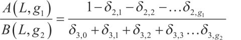 (5)
(5)
Next, consider Equation 2 again, applying ‘Wald’ to test the asymmetric impact of TR on EFP with null (H0): .png) + = -, where + =
+ = -, where + = .png) and - =
and - = .png) (from Equation 2).
(from Equation 2).
Short-term Relation: Asymmetry and Error Correction Towards Equilibrium
The section discusses short-run relations among the variables and tries to build an Error Correction Model, which corrects for short-run disequilibrium and traces the path towards long-run equilibrium (Equations 6 and 7 below)
 (6)
(6)
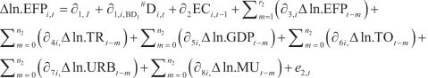
Equation 6 provides the short-run equation under ARDL (with a single structural break) with r2 being lags of EFP and n2 as lags of independent variables TR, GDP, TO, URB and MU, both follow AIC criteria. The term ECi,t-1 with coefficient .png) 2 represents the error correcting term, while 4,0 is the short-run price transmission elasticity coefficient from variable TR to EFP.
2 represents the error correcting term, while 4,0 is the short-run price transmission elasticity coefficient from variable TR to EFP.
Equation 7 provides an error correction and adjustment mechanism under NARDL with the TR variable decomposition as TR+ and TR– under a short-run framework.
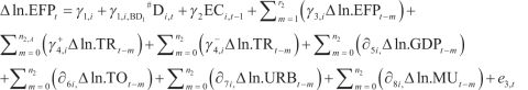 (7)
(7)
Further, for both equations, Equation 6 and 7, the term ECt-1 shows how fast the market would adjust to achieve long-run equilibrium, implying that a shock under the system has an adjustment mechanism as 2 (ARDL) and .png) 2 (NARDL). The ‘n’ period shock adjustment being 1-(1 – 2)n and 1-(1 – 2)n for two models, respectively.
2 (NARDL). The ‘n’ period shock adjustment being 1-(1 – 2)n and 1-(1 – 2)n for two models, respectively.
NARDL also provides useful information on short-run asymmetry, with null defined as .png) (from Equation 7).
(from Equation 7).
Results
This section summarises findings from Table 3,Table 4,Table 5,Table 6, Table 7, Table 8 and Table 9. Table 3 and Table 4 present BDS test results, indicating non-linearity in the EFP variable for both India and China.
The rejection of the null hypothesis across all embedding dimensions supports the use of non-linear models; ARDL (with structural break) and NARDL.
Table 4. BDS Results for Our Variable EFP (India).
Following this, Table 5 and Table 6 display results from the Partial F-Bounds test for long-run co-integration. For both India and China, and under both ARDL and NARDL models, the computed F-statistics exceeded upper bound at 1% level, confirming long-run co-integration.
Table 5. Partial ‘F’ Bounds Test ARDL (with Dummy) Model.
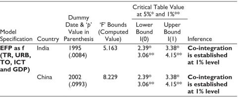
Notes: H0: 2 = 3 = 4 = 5 = 6 = 7 = 0 (see Equation 1)
Table Result: Co-integration is established for both India and China.
Dummy Coefficients included in ARDL were significant for India at 1% and for China at 10% justifying inclusion of structural break for India and partially justifying for China. The significance levels are 5%(*) and 1 %(**).
Table 6. Partial ‘F’ Bounds Test NARDL Model.
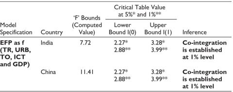
Notes: Ho: 2 = 3 = 4 = 5 = 6 = 7 = 0 (see Equation 2)
Table result: Co-integration is established for both India and China. The significance levels are 5%(*) and 1 %(**).
The co-integration established for India and China enabled long-run analysis. Table 7 shows that TR significantly and positively affects EFP in both countries, at 1% level for India and 10% for China. For India, ICT negatively impacts EFP, while in China, GDP, TO, and URB positively affect EFP, and ICT has a negative influence. These findings align with Hussain et al. (2023) and Salahuddin et al. (2016).
Table 7. Long-run Results Under Both ARDL and NARDL Model.
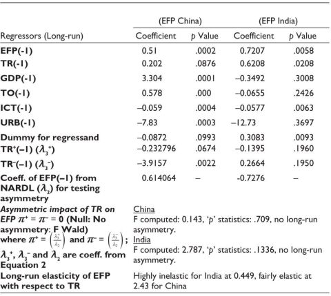
Notes: 1. Model selection method: AIC.
2. Model selected: China: ARDL (2, 0, 2, 1, 1, 2); India ARDL (1, 1, 2, 0, 2, 2); China NARDL (1, 0, 1, 0, 2, 2, 0); India NARDL (2, 2, 2, 2, 1, 2, 1).
3. For long-run elasticity of EFP with respect to TR, the applicable formula from Equation 5 is given as: .png)
The Wald F-test under NARDL confirmed no long-run asymmetry of TR on EFP in either country. Long-run elasticity of TR on EFP was highly inelastic for India (0.449) and fairly elastic for China (2.43), suggesting China’s gradual transition toward alternative fuels, while India remains reliant on fossil fuels.
In the short run (Table 8), TR, TO, and ICT impact EFP in India; TR and TO positively, ICT negatively. In China, all variables influence EFP, with ICT again showing a negative effect, and the rest of the variables positively. Short-run elasticity of TR on EFP remained inelastic in both nations, showing limited flexibility. No evidence of short-run asymmetry was seen under the study. The ECM(-1) term confirmed stable but slow adjustment: Faster in China than in India.
Table 8. Short-run Results and Error Correction.
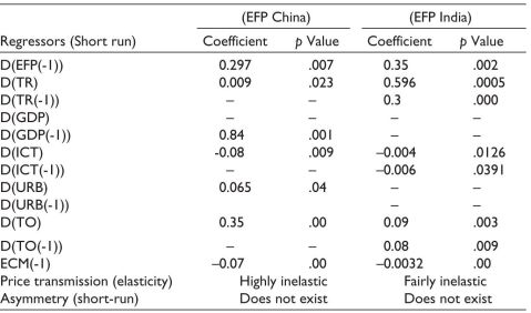
Notes: 1. Short-run elasticity of EFP w.r.t TR: We consider contemporaneous slope coefficients of the change variable TR.
2. Asymmetry is tested by equating the two terms: .png)
3. For error correction we consider lagged ECM term coefficient which must be negative and significant.
Table 9 presents diagnostics: Breakpoint ADF tests showed mixed stationarity across variables, justifying ARDL modelling. Results from BG-LM and BPG tests indicated no serial correlation or heteroscedasticity. These diagnostics support the reliability of the results.
Table 9. Diagnostics.
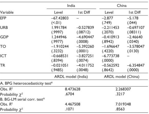
Notes: 1. Break date; EFP China was in 2002, and EFP India was in 1995.
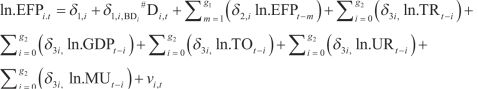
2. @.png) EFPt = 1 + 1* DEFP,t + (2 – 1)EFPt – 1 +
EFPt = 1 + 1* DEFP,t + (2 – 1)EFPt – 1 + .png) 3i, EFPt – i + ut, …, is the Breakpoint ADF test equation for variable EFP with single break point, EFPt is change in EFP in period t, 1, represents intercept, 1* DEFP,t being single break intercept, and Dummy taking value of ‘1’ for observations falling after break date of EFP and ‘0’ before. The break is validated if 1,* is statistically significant. Term EFPt – 1 tests for stationarity with (2 – 1) as coefficient, where ‘t’ computed is compared with ADF ‘t’ tau tables. Next term = 1 3i, ERPt – i removes serial correlation, and ut is the random error term. Using a similar methodology, we construct the stationary equation for our other remaining variables.
3i, EFPt – i + ut, …, is the Breakpoint ADF test equation for variable EFP with single break point, EFPt is change in EFP in period t, 1, represents intercept, 1* DEFP,t being single break intercept, and Dummy taking value of ‘1’ for observations falling after break date of EFP and ‘0’ before. The break is validated if 1,* is statistically significant. Term EFPt – 1 tests for stationarity with (2 – 1) as coefficient, where ‘t’ computed is compared with ADF ‘t’ tau tables. Next term = 1 3i, ERPt – i removes serial correlation, and ut is the random error term. Using a similar methodology, we construct the stationary equation for our other remaining variables.
#BPG Heteroscedasticity test first determines R2 of auxiliary equation ut2 = .png) 1+ 2 X2t + 3 X3t +…+ k Xkt, followed by n.R2aux ~
1+ 2 X2t + 3 X3t +…+ k Xkt, followed by n.R2aux ~ .png) 2m – 1.; Null: No heteroscedasticity, that is, 2 =3 = 4, …, = k = 0.
2m – 1.; Null: No heteroscedasticity, that is, 2 =3 = 4, …, = k = 0.
*BG-LM serial correlation: The test also constructs an auxiliary equation: uEFP = 1 + 2 EFPt – 1 + 3 EFPt – 2 +…+ p EFPt-p + .png) 1 uEFPt–1 + 2 uEFPt–2 …+ m uEFPt–m + et, number of lags of regression and error term being ‘p’ and ‘m’, respectively, ‘p’ > ‘m’. Null: 1 = 2 = …, m = 0 (no serial correlation between residuals). Reject the null when R2 (n-p) > 2m.
1 uEFPt–1 + 2 uEFPt–2 …+ m uEFPt–m + et, number of lags of regression and error term being ‘p’ and ‘m’, respectively, ‘p’ > ‘m’. Null: 1 = 2 = …, m = 0 (no serial correlation between residuals). Reject the null when R2 (n-p) > 2m.
Figures in parentheses are ‘p’ values.
Conclusion and Implications
This study empirically examined the long-term dynamic relationship between CO2 emissions from liquid fuel consumption in the TR and EFP in China and India, using ARDL and NARDL models. Co-integration was confirmed at a 1% significance level for both countries. In the long run, TR had a positive impact on EFP; highly inelastic for India and somewhat elastic for China. No asymmetric impact of TR on EFP was detected.
In the short run, TR also influenced EFP with inelastic elasticity in both countries. The ECM(-1) coefficient was negative and stable, indicating adjustment toward equilibrium; moderate (7% p.a.) for China and very slow (0.3% p.a.) for India.
Three key observations emerge: (a) the absence of asymmetry may stem from limited negative growth years in TR and the composite nature of EFP; (b) elasticity contrasts: India’s inelastic versus China’s elastic long-run TR-EFP link; and (c) different speeds of long-run adjustment.
These findings do provide valuable policy insights. India’s slower pace suggests time for planning sustainable transport policies. China’s relatively elastic long-run response and faster adjustment indicate better readiness for energy transition. For both nations, inelastic short-run elasticity highlights challenges like poor substitutability and infrastructure gaps. Thus, long-term planning is essential, especially for India, where short- and long-run patterns show little divergence.
Declaration of Conflicting Interests
The authors declared no potential conflicts of interest with respect to the research, authorship and/or publication of this article.
Funding
The authors received no financial support for the research, authorship and/or publication of this article.
ORCID iD
Rakesh Shahani https://orcid.org/0000-0003-4916-2740
Abbes, S., & Bulteau, J. (2018). Growth in transport sector CO2 emissions in Tunisia: An analysis using a bounds testing approach. International Journal of Global Energy Issues, 41(1–4), 176–197.
Acheampong, A. O., Dzator, J., Dzator, M., & Salim, R. (2022). Unveiling the effect of transport infrastructure and technological innovation on economic growth, energy consumption and CO2 emissions. Technological Forecasting and Social Change, 182, 121843.
Amri, F., Zaied, Y. B., & Lahouel, B. B. (2019). ICT, total factor productivity, and carbon dioxide emissions in Tunisia. Technological Forecasting and Social Change, 146, 212–217.
Asongu, S. A., Le Roux, S., & Biekpe, N. (2017). Environmental degradation, ICT and inclusive development in Sub-Saharan Africa. Energy Policy, 111, 353–361.
Ayadi, A., & Hammami, S. (2015). Analysis of the technological features of regional public transport companies: The Tunisian case. Public Transport, 7, 429–455.
Brock, W. A., Dechert, W., & Scheinkman, J. (1987). A test for independence based on the correlation dimension [Working paper]. University of Wisconsin–Madison, University of Houston, and University of Chicago.
Brown-Steiner, B., Hess, P., Chen, J., & Donaghy, K. (2016). Black carbon emissions from trucks and trains in the Midwestern and Northeastern United States from 1977 to 2007. Atmospheric Environment, 129, 155–166.
Charfeddine, L. (2017). The impact of energy consumption and economic development on ecological footprint and CO2 emissions: Evidence from a Markov switching equilibrium correction model. Energy Economics, 65, 355–374.
Charfeddine, L., & Khediri, K. B. (2016). Financial development and environmental quality in UAE: Cointegration with structural breaks. Renewable and Sustainable Energy Reviews, 55, 1322–1335.
Charfeddine, L., & Mrabet, Z. (2017). The impact of economic development and social-political factors on ecological footprint: A panel data analysis for 15 MENA countries. Renewable and Sustainable Energy Reviews, 76, 138–154.
Churchill, S. A., Inekwe, J., Ivanovski, K., & Smyth, R. (2021). Transport infrastructure and CO2 emissions in the OECD over the long run. Transportation Research Part D: Transport and Environment, 95, 102857.
Frey, S. D., Harrison, D. J., & Billett, E. H. (2006). Ecological footprint analysis applied to mobile phones. Journal of Industrial Ecology, 10(1–2), 199–216.
Global Footprint Network. (2023). Footprint data platform. Retrieved, 21 September 2025, from http://data.footprintnetwork.org
Hassan, S. T., Xia, E., Khan, N. H., & Shah, S. M. A. (2019). Economic growth, natural resources, and ecological footprints: Evidence from Pakistan. Environmental Science and Pollution Research, 26, 2929–2938.
Hussain, M. M., Pal, S., & Villanthenkodath, M. A. (2023). Towards sustainable development: The impact of transport infrastructure expenditure on the ecological footprint in India. Innovation and Green Development, 2(2), 100037.
IRENA. (2021). Renewable energy policies for cities: Buildings. https://www.irena.org/-/media/Files/IRENA/Agency/Publication/2021/May/IRENA_Policies_for_Cities_Buildings_2021.pdf
Nasreen, S., Mbarek, M. B., & Atiq-ur-Rehman, M. (2020). Long-run causal relationship between economic growth, transport energy consumption and environmental quality in Asian countries: Evidence from heterogeneous panel methods. Energy, 192, 116628.
Nathaniel, S., & Khan, S. A. R. (2020). The nexus between urbanization, renewable energy, trade, and ecological footprint in ASEAN countries. Journal of Cleaner Production, 272, 122709.
OECD. (2021). Green growth indicators. OECD Publishing.
Perron, P. (1994). Trend, unit root and structural change in macroeconomic time series. In Cointegration: For the applied economist (pp. 113–146). Palgrave Macmillan.
Pesaran, M. H., Shin, Y., & Smith, R. J. (2001). Bounds testing approaches to the analysis of level relationships. Journal of Applied Econometrics, 16(3), 289–326.
Pradhan, R. P., Nair, M. S., Hall, J. H., & Bennett, S. E. (2024). Planetary health issues in the developing world: Dynamics between transportation systems, sustainable economic development, and CO2 emissions. Journal of Cleaner Production, 449, 140842.
Saboori, B., Sapri, M., & Baba, M. B. (2014). Economic growth, energy consumption and CO2 emissions in OECD’s transport sector: A fully modified bi-directional relationship approach. Energy, 66, 150–161.
Salahuddin, M., Alam, K., & Ozturk, I. (2016). The effects of internet usage and economic growth on CO2 emissions in OECD countries: A panel investigation. Renewable and Sustainable Energy Reviews, 62, 1226–1235.
Santos, G. (2017). Road transport and CO2 emissions: What are the challenges? Transport Policy, 59, 71–74.
Sasana, H., & Aminata, J. (2019). Energy subsidy, energy consumption, economic growth, and carbon dioxide emission: Indonesian case studies. International Journal of Energy Economics and Policy, 9(2), 117–122.
Satrovic, E., Cetindas, A., Akben, I., & Damrah, S. (2024). Do natural resource dependence, economic growth and transport energy consumption accelerate ecological footprint in the most innovative countries? The moderating role of technological innovation. Gondwana Research, 127, 116–130.
Shabani, Z. D., & Shahnazi, R. (2019). Energy consumption, carbon dioxide emissions, information and communications technology, and gross domestic product in Iranian economic sectors: A panel causality analysis. Energy, 169, 1064–1078.
Shang, W. L., Ling, Y., Ochieng, W., Yang, L., Gao, X., Ren, Q., Chen, Y., & Cao, M. (2024). Driving forces of CO2 emissions from the transport, storage and postal sectors: A pathway to achieving carbon neutrality. Applied Energy, 365, 123226.
Sheng, P., & Guo, X. (2016). The long-run and short-run impacts of urbanization on carbon dioxide emissions. Economic Modelling, 53, 208–215.
Shin, Y., Yu, B., & Greenwood-Nimmo, M. (2014). Modelling asymmetric cointegration and dynamic multipliers in a nonlinear ARDL framework. In Festschrift in honor of Peter Schmidt (pp. 281–314). Springer.
Strand, R., Kovacic, Z., Funtowicz, S., Benini, L., & Jesus, A. (2021). Growth without economic growth. European Environment Agency , 1–13. doi:10.2800/492717.
UN Fact Sheet. (2021, October). Fact sheet on climate change. UN Sustainable Transport Conference, Beijing. https://www.un.org/sites/un2.un.org/files/2021/10/fact_sheet_transport_general.pdf
World Bank. (2023). World development indicators. World Bank Group. https://databank.worldbank.org/source/world-development-indicators?utm
